


R client package to access the web service API of the KorAP Corpus Analysis Platform developed at IDS Mannheim
library(RKorAPClient)
KorAPConnection(verbose=TRUE) |> corpusQuery("Hello world") |> fetchAll()
Interactive time-series plots using highcharter
For an interactive frequency plot over time with confidence intervals, pass the result of frequencyQuery() directly to hc_freq_by_year_ci(). This helper is provided by RKorAPClient and returns an interactive HTML widget, with tooltips and clickable data points that open the corresponding KorAP search results. No additional plotting package needs to be loaded. By default, it shows frequencies per million tokens; the example below uses as.alternatives = TRUE to show percentages instead.
See the Highcharts license notes below.
library(RKorAPClient)
query = c("macht []{0,3} Sinn", "ergibt []{0,3} Sinn")
years = c(1980:2010)
as.alternatives = TRUE
vc = "textType = /Zeit.*/ & creationDate in"
KorAPConnection(verbose = TRUE) |>
  frequencyQuery(query, paste(vc, years), as.alternatives = as.alternatives) |>
  hc_freq_by_year_ci(as.alternatives)
You can turn on verbose logging globally without changing calls by setting an environment variable (or an R option):
# Environment variable (recommended for sessions / ~/.Renviron)
Sys.setenv(KORAP_VERBOSE = "true")
KorAPConnection()  # uses verbose = TRUE

# Alternatively, R option
options(rkorap.verbose = TRUE)
KorAPConnection()
Explicit verbose arguments still take precedence over these settings.
Use RStudio's Stop button or your R interface's interrupt key (Escape or Ctrl+C) to stop the running script and return to the console.
To speed up repeated analyses and to avoid unnecessary load on the KorAP servers, API responses are cached locally by default, in the cache directory that is standard for your operating system (see R.cache). Cached responses are invalidated automatically when the corpus index revision changes.
kco <- KorAPConnection(cache = FALSE)  # do not cache anything in this connection
clearCache()                           # discard all locally cached responses
This cache is a transparent speed-up that you can throw away at any time. To keep a finished result in a file of your own instead, see the cacheAs parameter described further below.
Please note that, in the case of DeReKo, authorized queries behave differently inside and outside the IDS, because of the special license situation. Cached results do not record from where a request was issued, so if you get unexpected results after changing networks, use clearCache() or cache = FALSE.
The client sends the virtual-corpus definition (vc) to the selected KorAP instance. Available metadata fields, their meaning and their coverage depend on that corpus; the client cannot decide which field answers your research question.
pubDaterefers to publication, whereascreationDaterefers to text creation. They are not generally interchangeable. For a question about publication years, usepubDate; for creation years, usecreationDate, after checking how the corpus defines and populates the field.- A publication date may describe the edition represented in the corpus, rather than the first publication of the work. A creation date is not automatically a documented date of first publication either.
- The two fields may give the same results in one corpus or subset. Do not assume that this carries over to another corpus, particularly when moving between DeLiKo and DeReKo.
Check the corpus documentation for the intended meaning, missing values and date precision. textMetadata() (see below) shows stored values for individual texts; it does not supply field definitions or a complete inventory of possible values. A syntactically valid query and plausible counts do not establish that the right metadata field was chosen. The need for accessible field descriptions is also discussed in Kalamar issue #40.
The time-series examples use creationDate; their year axis therefore follows that field, not necessarily publication year.
library(RKorAPClient)
library(ggplot2)
kco <- KorAPConnection(verbose = TRUE)

expand_grid(
  ressort = c(
    Wirtschaft = "idsColumn = /Wirtschaft.*/",
    `Nicht-Wirtschaft` = "idsColumn != /Wirtschaft.*/"
  ),
  year = 2002:2018
) |>
  mutate(
    frequencyQuery(kco, "[tt/l=Heuschrecke]",
      paste(ressort, "& creationDate in", year)),
    ressort = names(ressort)
  ) |>
  ipm() |>
  ggplot(aes(year, ipm, fill = ressort, colour = ressort)) +
  theme_minimal() +
  geom_freq_by_year_ci() +
  labs(x = "Jahr", y = "Relative Häufigkeit (IPM)",
       fill = "Ressort", colour = "Ressort")
frequencyQuery returns a data frame with raw frequencies (in totalResults), relative frequencies (in f), and confidence intervals. The relative frequencies and confidence limits are proportions, not values per million. Use ipm() when a plotting workflow needs values per million, as in the ggplot2 example above. When using hc_freq_by_year_ci(), pass the frequencyQuery() result directly: that helper performs the conversion itself (or converts to percentages with as.alternatives = TRUE). Calling ipm() first would scale the confidence limits twice.
For curved connections between annual observations, use
geom_freq_by_year_ci(smooth = TRUE). The measured years
remain visible as points; the curve and confidence-band boundaries are
interpolated for display only. Missing years leave gaps. This is not a trend
analysis, and the band does not provide confidence intervals for unobserved
dates. Interpolation follows the plot scales, including logarithmic axes.
For an interactive bar chart comparing frequencies between corpora or queries,
pass the unconverted frequencyQuery() result to hc_freq_bar_ci(). Like
hc_freq_by_year_ci(), this helper converts frequencies and confidence limits
to instances per million tokens automatically. Do not call ipm() or percent()
first. No additional plotting package needs to be loaded, and plotting stored
results makes no further requests to KorAP. Click a bar to open its concordances.
library(RKorAPClient)
kco <- KorAPConnection("https://korap.dnb.de")
frequencyQuery(kco, "Berlin",
  vc = c(Buchpreis = "award=buchpreis", DeLiKo = "")) |>
  hc_freq_bar_ci()
Named virtual corpora supply the category labels. A single query is compared across corpora; multiple queries in one corpus are compared across queries:
frequencyQuery(kco, c("Iowa", "Berlin"), vc = "award=buchpreis") |>
  hc_freq_bar_ci(horizontal = FALSE)
With multiple queries and multiple corpora, the chart groups queries within
each corpus. Set expand = TRUE in frequencyQuery() to request every
query/corpus combination, including when the two vectors have equal lengths.
Missing combinations and undefined frequencies remain gaps, while a zero-hit
query in a non-empty corpus retains its confidence interval. Supplied
confidence limits are preserved, including a custom conf.level.
For percentages of mutually exclusive, exhaustive alternatives, set
as.alternatives = TRUE in frequencyQuery(). The Highcharts helpers inherit
this recorded mode and reject a conflicting plotting argument. They retain
the original denominators when only some result rows are displayed. For older
tables without the recorded mode, specify it in the plotting call as well.
Use hc_freq_bar_ci(log = TRUE) for a logarithmic axis: zero frequencies and
intervals touching zero cannot be represented and are explicitly omitted.
Use highcharter functions to customize the returned widget.
Run demo("writtenVsSpoken_highcharts") for the spoken/written comparison.
Use showCI = FALSE to omit confidence intervals from frequency plots and
their tooltips. The option is available in hc_freq_bar_ci(),
hc_freq_by_year_ci(), geom_freq_bar_ci() and geom_freq_by_year_ci();
its default is TRUE. Observed frequencies are retained, and confidence-limit
columns are not required when intervals are disabled.
For a static figure suitable for print, use geom_freq_bar_ci(), the bar-chart
counterpart of geom_freq_by_year_ci(). It combines columns and aligned error
bars in a normal ggplot. Convert the frequencies and confidence limits with
ipm() once before plotting; this ggplot layer does not perform the automatic
conversion used by hc_freq_bar_ci().
library(RKorAPClient)
library(ggplot2)

p <- KorAPConnection("https://korap.dnb.de") |>
  frequencyQuery("Berlin",
    vc = c(Buchpreis = "award=buchpreis", DeLiKo = "")) |>
  ipm() |>
  ggplot(aes(x = label, y = ipm)) +
  geom_freq_bar_ci() +
  labs(x = NULL, y = "Instances per million tokens") +
  theme_bw()

p
ggsave("berlin.pdf", plot = p, width = 6, height = 4)
Map fill and group to the query variable for grouped comparisons. Bars and
intervals use the same dodge width. Explicit groups retain their positions
when colours or fills are overridden for monochrome printing. Use
coord_flip() for horizontal bars, or map aes(x = ipm, y = label) with
geom_freq_bar_ci(orientation = "y"). Ordinary ggplot themes, scales, facets
and exports work as usual. For alternatives, use as.alternatives = TRUE in
frequencyQuery() and percent() instead of ipm() before plotting.
The layer preserves supplied confidence limits and does not query KorAP.
Add idsThemeR::theme_ids() and idsThemeR::scale_fill_ids() for IDS styling;
mapped colours can use idsThemeR::scale_colour_ids().
Set the first (KorAPUrl) argument of the KorAPConnection function to the URL of the KorAP instance, providing the desired corpus, e.g. to
https://korap.ids-mannheim.de/instance/wiki/for the current German Wikipedia corpus provided by the IDShttps://korap.ids-mannheim.de/instance/english/for an English Wikipedia corpus provided by the IDShttps://korap.dnb.de/for the DeLiKo@DNB-XL German fiction corpushttps://korap.racai.ro/for the Contemporary Corpus of the Romanian Language (CoRoLa)
library(RKorAPClient)
KorAPConnection(KorAPUrl = "https://korap.ids-mannheim.de/instance/wiki/", verbose = TRUE) |>
  corpusQuery("Berlin") |>
fetchAll()corpusStats reports the size of the whole corpus or of a virtual corpus:
library(RKorAPClient)
kco <- KorAPConnection(verbose = TRUE)
corpusStats(kco, vc = "pubDate since 2020")
<KorAPCorpusStats>
The virtual corpus described by "pubDate since 2020" contains 3,942,948,561 tokens
in 253,752,552 sentences in 13,857,981 documents.
Passing a named vector of virtual corpora returns one row per corpus, labelled by the names you chose for them in a label column. frequencyQuery and collocationScoreQuery label their results the same way:
corpusStats(kco, vc = c(before = "pubDate until 2009", since = "pubDate since 2010"), as.df = TRUE)With as.df = TRUE you get a one row data frame with tokens, sentences, paragraphs and documents columns instead, which makes it easy to compare several virtual corpora.
The query language (Poliqarp+) and the definitions of virtual corpora mark regular expressions differently, and double quotes mean opposite things in them:
| query (Poliqarp+) | virtual corpus (vc) |
|
|---|---|---|
| regular expression | "…", e.g. [tt/l="(Frau|Mann)"] |
/…/, e.g. textType = /.*Krimi.*/ |
| literal string | '…' |
"…" |
KorAPConnection("https://korap.dnb.de") |>
  frequencyQuery('[tt/l="(Frau|Mann)"]', vc = "textType = /.*Krimi.*/")
In a query, / separates foundry and layer, as in tt/l, and is no regex delimiter. In a vc, textType = "Krimi.*" is no error, but looks for the literal string and finds nothing. Both follow the regular expression syntax of Lucene 5, not the Perl-style one of most programming languages. A regular expression has to match the whole value, hence the .* around Krimi. Inline flags, like (?i) for ignoring case, are not supported, so spell out case variants, e.g. [Kk]rimi. Nor are shorthand classes: \d stands for just the letter d, so write [0-9] instead.
Complex queries can take minutes on a large corpus, especially on DeLiKo@DNB (https://korap.dnb.de), or exceed the time limit of the server, in which case RKorAPClient warns that the results are incomplete. As long as KorAP does not offer sampling by itself, you can work around this, if relative frequencies are what you are after, by restricting the virtual corpus to a pseudo-random sample of texts, selected by the last digit of their text sigle (e.g. A00/JUN/39609):
vc |
sample of texts |
|---|---|
textSigle = /.*5/ |
about 10 % |
textSigle = /.*[0-4]/ |
about 50 % |
KorAPConnection("https://korap.dnb.de", verbose = TRUE) |>
  frequencyQuery("[orth=mit] [orth=einer]", vc = "textSigle = /.*5/")
The relative frequency f remains an estimate for the whole (virtual) corpus, with a correspondingly wider confidence interval, whereas totalResults counts only the hits in the sample. Combine the sample with other conditions using &, e.g. vc = "textType = /.*Krimi.*/ & textSigle = /.*5/". Each digit selects a different sample, and always the same one, so results stay reproducible.
How much time a sample saves depends on whether the server has recently read the index of the query terms, for whatever query. If not, it saves hardly any, because most of the time goes into reading the index from disk: in DeLiKo@DNB, the query above took 35 seconds on the 10 % sample, about as long as a comparable query on the whole corpus. If so, it saves about as much as it leaves out: the same query took 0.9 seconds on another 10 % sample and 6.6 seconds on the whole corpus. A sample therefore pays off in series of queries on the same terms, such as a frequencyQuery over many years or a collocationAnalysis. Repeating a query on the same vc takes no time anyway, as its result comes from the local cache. Queries that are fast anyway do not get faster, because selecting the sample takes some time itself.
textMetadata retrieves all metadata KorAP holds for a text, given its sigle as found in the textSigle column of query results:
KorAPConnection() |> textMetadata("WPD17/L79/98721")| textSigle | author | title | pubDate | textType |
|---|---|---|---|---|
| WPD17/L79/98721 | GeorgDerReisende, u.a. | Leverone | 2017-07-01 | Enzyklopädie |
The result has one column per metadata field the corpus provides – 26 in this example, so the table above shows only a selection.

Are Nutzer*innen and Nutzer:innen similarly dispersed across press sources, publication countries and years, allowing for the size of each group?
kco <- KorAPConnection()
queries <- c("Nutzer*innen" = "[orth='Nutzer*innen']",
             "Nutzer:innen" = "[orth='Nutzer:innen']")
hits <- corpusQuery(kco, queries,
  vc = "pubDate since 2023 & pubDate until 2025 & textType=/Zeit.*/ & pubPlaceKey=/.+/",
  fields = c("corpusTitle", "pubPlaceKey", "pubDate")) |>
  fetchSamplePages(maxHits = Inf, seed = 7)
d <- dispersionAnalysis(hits, by = c("source", "pubPlaceKey", "year"))
print(d)
hc_dispersion(d, partition = "source", top = 12)
The library obtains group sizes and includes groups without hits. The table compares the spellings side by side; the chart compares hit shares with corpus token shares. Smaller DP/DPnorm and larger D/D2/S indicate more even distributions, but measures can disagree. Compare spellings within the same partition; dispersion across years is not a trend test.
maxHits = Inf fetches all hits. For a smaller exploratory dataset, use
maxHits = 2000: this samples pages, not independent hits, and can strongly
bias dispersion estimates.
See ?dispersionAnalysis for grouping and sampling options,
?defaultDispersionFunctions for measure definitions, interpretation and
references, and demo("dispersion") for the complete example. Custom measures
can be supplied through scoreFunctions. The measures follow
Gries (2020); see also
his companion resources.
While collocationAnalysis searches for collocates, collocationScoreQuery computes association scores for pairs you already have in mind. It accepts a vector of collocates and queries every combination of collocate and virtual corpus:
KorAPConnection() |>
collocationScoreQuery("Grund", c("triftiger", "guter", "Berlin"))| node | collocate | O | E | logDice | pmi | ll |
|---|---|---|---|---|---|---|
| Grund | triftiger | 2390.50 | 6.31 | 3.96 | 8.57 | 23808.61 |
| Grund | guter | 12902.50 | 2713.24 | 6.06 | 2.25 | 19868.49 |
| Grund | Berlin | 7865.50 | 26212.26 | 3.84 | -1.74 | 17766.78 |
O is the observed and E the expected co-occurrence frequency. Triftiger is by far the most strongly attracted of the three (highest pmi), while Berlin co-occurs with Grund less often than chance would predict, which is what a negative pmi expresses. logDice, in contrast, does not compare against an expected frequency but relates the co-occurrence frequency to how often the two words occur at all, which is why the frequent guter Grund leads there – and why Berlin, although it co-occurs with Grund less often than expected, still scores nearly as high as triftiger. collocationAnalysis therefore discards collocates occurring less often than expected by default, which its minObservedExpectedRatio parameter controls. collocationScoreQuery does not filter, since here the pairs to score are asked for explicitly – which is why Berlin is shown above.
library(RKorAPClient)
library(knitr)
KorAPConnection(verbose = TRUE) |> auth() |>
  collocationAnalysis(
    "focus(in [tt/p=NN] {[tt/l=setzen]})",
    leftContextSize = 1,
    rightContextSize = 0,
    exactFrequencies = FALSE,
    searchHitsSampleLimit = 1000,
    topCollocatesLimit = 20
  ) |>
  mutate(LVC = sprintf("[in %s setzen](%s)", collocate, webUIRequestUrl)) |>
  select(LVC, logDice, pmi, ll) |>
  head(10) |>
  kable(format="pipe", digits=2)
The focus, here, with the [tt/l=setzen] in braces, makes sure that the left context size parameter 1 is understood relative to the lemma setzen.
The [tt/p=NN] in the focus query makes sure that only nouns (at this position) are considered as collocates.
To perform a simple collocation analysis for a word form, rather than a lemma and without restriction to light verb constructions, simply use, for instance, KorAPConnection(verbose = TRUE) |> auth() |> collocationAnalysis("setzte").
For a lemma, either put the lemma layer into the query itself, collocationAnalysis("[tt/l=setzen]"), or let lemmatizeNodeQuery = TRUE build that query from the word form: collocationAnalysis("setzen", lemmatizeNodeQuery = TRUE).
| LVC | logDice | pmi | ll |
|---|---|---|---|
| in Szene setzen | 9.66 | 10.86 | 465467.52 |
| in Gang setzen | 9.21 | 10.57 | 256146.92 |
| in Verbindung setzen | 8.46 | 9.62 | 189682.19 |
| in Kenntnis setzen | 8.28 | 9.81 | 101112.02 |
| in Bewegung setzen | 8.11 | 9.24 | 149397.91 |
| in Brand setzen | 8.10 | 9.33 | 122427.05 |
| in Anführungszeichen setzen | 7.50 | 11.96 | 33959.99 |
| in Kraft setzen | 6.88 | 7.88 | 77796.85 |
| in Marsch setzen | 6.87 | 9.27 | 22041.63 |
| in Klammern setzen | 6.55 | 10.08 | 15643.27 |
Collocation analyses can take a while, and comparing them across virtual corpora, as shown below, multiplies that. With the cacheAs parameter you can have the result stored in an RDS file of your choice, so that repeated calls – when re-knitting a document, for example – return the cached result immediately instead of querying the server again:
KorAPConnection(verbose = TRUE) |> auth() |>
collocationAnalysis("Ameisenplage", cacheAs = "ameisenplage-ca.rds")frequencyQuery, corpusStats, collocationScoreQuery and textMetadata take the parameter as well, where it is less about time: the file keeps the numbers a text was written about, which KorAP would answer differently once the corpus has grown, and it lets the script run again without a server at all. A file is only reused for the call that produced it – a changed parameter, a different KorAP instance, or a version of RKorAPClient whose scores differ has it recomputed and overwritten, with a warning saying why.
Consider keeping such a file under version control next to the document that uses it, so that the analysis travels with the text. cacheAsInfo() reads back what produced it: parameters, KorAP instance, index revision and package version.
When a file is refused although you know it to be sound – one written by a development version that already had the current scores, say – blessCacheAs("klima.rds") vouches for it once and for good. And when there is no time to recompute anything at all, withCachedResults({ ... }) takes the files as they are for the code inside it, with mode = "offline" refusing to query the server even for a file that is missing:
withCachedResults(mode = "offline", {
  ca <- kco |> collocationAnalysis("Klima", cacheAs = "klima-ca.rds")
})If you pass a named vector of virtual corpora as vc, collocationAnalysis compares the collocates of the node between them and adds a set of comparison columns, labelled with the names you provided:
library(RKorAPClient)
library(dplyr)

ca <- KorAPConnection(verbose = TRUE) |> auth() |>
  collocationAnalysis(
    "Klima",
    vc = c(Nullerjahre = "creationDate since 2000 & creationDate until 2009",
           Zehnerjahre = "creationDate since 2010 & creationDate until 2019"),
    leftContextSize = 1,
    rightContextSize = 1,
    exactFrequencies = FALSE,
    searchHitsSampleLimit = 2000,
    topCollocatesLimit = 20
  )

ca |>
  filter(label == "Zehnerjahre", !imputed) |>
  arrange(desc(delta_logDice)) |>
  select(collocate, logDice_Nullerjahre, logDice_Zehnerjahre, delta_logDice, winner_logDice)
Besides the usual association scores, the result then contains, for each score:
<score>_<label>– the score of the collocate in the respective virtual corpus,delta_<score>andmax_delta_<score>– the difference between the compared corpora,winner_<score>/loser_<score>– the label in which the collocate is most / least characteristic, each with a corresponding_valueand_webUIRequestUrlcolumn that links directly to the concordances in the KorAP web interface,imputed,n_imputedandimputed_<label>– markers for collocates that were attested in one of the compared corpora only.
Two properties are worth knowing when working with these columns:
- The result holds one row per collocate and virtual corpus, with the comparison columns repeated identically on each of them. Filter on
label, as above, to get one row per collocate. - Collocates that pass the
minOccurandtopCollocatesLimitthresholds in one virtual corpus but not in the other have no observed score for the latter. Such cells are imputed from a floor value, so theirdelta_*measures the distance to that floor rather than an attested difference.filter(!imputed)restricts the comparison to collocates attested everywhere, andqueryMissingScores = TRUEretrieves the missing scores from the server instead.
Since the labels become part of the column names, plain syntactic names work best – a label starting with a digit, for instance, ends up prefixed with X. The names and semantics of the comparison columns are still experimental and may change without a deprecation cycle; ?collocationAnalysis documents them in full, including how to read them.
In order to perform collocation analysis and other textual queries on corpus parts for which KWIC access requires a login, you need to authorize your application with an access token.
What a token buys is KWIC access, not the query itself. Frequencies are counted over the whole corpus either way, so frequencyQuery(), corpusStats() and collocationScoreQuery() need no authorization even on DeReKo – the very first example above queries it unauthorized. What an unauthorized application does not receive are the KWIC snippets of copyrighted texts, which is why corpusQuery() with metadataOnly = FALSE and collocationAnalysis(), which reads those snippets, do need one there.
Even that is a matter of the individual text's license rather than of the corpus: DeReKo's freely licensed parts, the Wikipedia corpora among them, hand out their snippets to anyone. Some instances are liberally licensed throughout and need no authorization at all – the German and English Wikipedia talk pages at https://korap.ids-mannheim.de/instance/wiki and https://korap.ids-mannheim.de/instance/english, both under a Creative Commons license, return KWIC snippets to a plain KorAPConnection().
In the case of DeReKo, authorization can be done in three different ways.
Authorize your RKorAPClient application via the usual OAuth browser flow using the default application id and the auth method:
kco <- KorAPConnection() |> auth()(Required for headless operation, e.g. in batch scripts)
-
Log in into the KorAP DeReKo instance
-
Open the KorAP OAuth settings
-
If you have not yet registered a client application, or not the desired one, register one (it is sufficient to fill in the marked fields).
-
Click the intended client application name.
-
If you do not have any access tokens yet, click on the "Issue new token" button.
-
Copy one of your access tokens to you clipboard by clicking on the copy symbol ⎘ behind it.
-
In R/RStudio, paste the token into your KorAPConnection initialization, overwriting
<access token>in the following example:kco <- KorAPConnection(accessToken="<access token>")
The whole process is shown in this video:
RKorAPClient-get-and-persists-accessToken.mp4
Authorize your RKorAPClient application via the usual OAuth browser flow, using your own application id and the auth method:
- Follow steps 1-4 of the old way shown above.
- Click on the copy symbol ⎘ behind the ID of your client application.
- Paste your clipboard content overwriting
<application ID>in the following example code:kco <- KorAPConnection() |> auth(app_id = "<application ID>")
(Not recommended for the default application id, as it is not secure.)
You can also persist the access token for subsequent sessions with the persistAccessToken function:
persistAccessToken(kco)Afterwards a simple kco <- KorAPConnection() will retrieve the stored token.
Piping the result through the auth() function kco <- KorAPConnection() |> auth() works and does nothing, in this case.
To use the access token for simple corpus queries, i.e. to make corpusQuery return KWIC snippets, the metadataOnly parameter must be set to FALSE, for example:
corpusQuery(kco, "Ameisenplage", metadataOnly = FALSE) |> fetchAll()should return KWIC snippets, if you have authorized your application successfully.
You can use complex annotation queries in all client functions just as in the KorAP web interface (see KorAP Query Help). To fetch the annotations for all matches in a KorAPQuery object, use the fetchAnnotations() method:
library(RKorAPClient)
kco <- KorAPConnection(verbose = TRUE) |> auth()
q <- corpusQuery(kco, "[marmot/p=ADJA] [tt/l=Ameisenplage & marmot/m=case:acc]", metadataOnly = FALSE) |>
  fetchAll() |>
  fetchAnnotations(foundry = "marmot")

View(cbind(q@collectedMatches[c("textSigle", "snippet")],
           pos = q@collectedMatches$pos,
           morph = q@collectedMatches$morph))
The annotations are stored in q@collectedMatches$pos, q@collectedMatches$morph, and q@collectedMatches$lemma (for foundries that contain lemma annotations, like tt, but not marmot).
Small workflows you may find useful:
# 1) Add TT (POS/lemma), then add MarMoT (morph) without overwriting
q <- corpusQuery(kco, "Ameisenplage", metadataOnly = FALSE) |>
  fetchAll() |>
  fetchAnnotations(foundry = "tt") |>
  fetchAnnotations(foundry = "marmot")  # keeps TT POS/lemma, adds morph

# 2) Force re-fetch to repair damaged annotations
q <- fetchAnnotations(q, foundry = "tt", overwrite = TRUE)Tip: If you don't know any of the provided query languages or the tag sets, you can use KorAP's query by example (or rather query by match) feature by searching for a concrete example of the construction you are interested in, and then constructing your complex annotation query by just clicking on the entries in the tokens annotations of the query results, as demonstrated in this video (see also Diewald/Barbu Mititelu/Kupietz 2019).
More elaborate R scripts demonstrating the use of the package can be found in the demo folder.
- Install latest R version for your OS, following the instructions from CRAN
- Download and install latest RStudio Desktop from RStudio downloads
# Debian, Ubuntu, ...
sudo apt -f install # install possibly missing RStudio dependencies
sudo apt install r-base-dev r-cran-rcpp r-cran-cpp11 libcurl4-openssl-dev libxml2-dev libsecret-1-dev libfontconfig1-dev libssl-dev

# Fedora, CentOS, RHEL, Rocky Linux, AlmaLinux, ...
sudo dnf install R-devel libcurl-devel openssl-devel libxml2-devel libsecret-devel fontconfig-devel

# Arch Linux
pacman -S base-devel gcc-fortran libsodium curlStart RStudio and click on Install Packages… in the Tools menu. Enter RKorAPClient in the Packages input field and click on the Install button (keeping Install Dependencies checked).
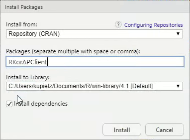
If the installation fails for some reason, you might need to update your installed R packages first (Tools -> Check for Package Updates, Select All, Install Updates).
Start R, then install RKorAPClient from CRAN (or development version from GitHub or KorAP's gerrit server).
install.packages("RKorAPClient")remotes::install_github("KorAP/RKorAPClient")full-install-on-mac.mp4
RKorAPClient-install-on-Ubuntu.mp4
Authors: Marc Kupietz, Nils Diewald
Contributors: Tim Feldmüller
Copyright (c) 2026, Leibniz Institute for the German Language, Mannheim, Germany
This package is developed as part of the KorAP Corpus Analysis Platform at the Leibniz Institute for German Language (IDS).
It is published under the BSD-2 License.
The KorAP logo was designed by Norbert Cußler-Volz and is released under the terms of the Creative Commons License BY-NC-ND 4.0.
RKorAPClient imports parts of the highcharter package which has a dependency on Highcharts, a commercial JavaScript charting library. Highcharts offers both a commercial license as well as a free non-commercial license. Please review the licensing options and terms before using the highcharter plot options, as the RKorAPClient license neither provides nor implies a license for Highcharts.
Highcharts is a Highsoft product which is not free for commercial and governmental use.
By using RKorAPClient you agree to the respective terms of use of the accessed KorAP API services which will be printed upon opening a connection (KorAPConnection(...).
Contributions are very welcome!
Your contributions should ideally be committed via our Gerrit server to facilitate reviewing (see Gerrit Code Review - A Quick Introduction if you are not familiar with Gerrit). However, we are also happy to accept comments and pull requests via GitHub.
Please note that unless you explicitly state otherwise any contribution intentionally submitted for inclusion into this software shall – as this software itself – be under the BSD-2 License.
Part of the test suite prompts current LLMs with this Readme and checks that the code they write from it uses the package correctly, so that a gap in the documentation shows up as a failing test – see Kupietz et al. (2026) on the approach. These tests run only when RKORAP_LLM_MODELS explicitly selects models (or default) and the corresponding API keys are available. See the test-suite guide for details.
- Diewald, Nils/Barbu Mititelu, Verginica/Kupietz, Marc (2019): The KorAP user interface. Accessing CoRoLa via KorAP. In: On design, creation and use of the Reference Corpus of Contemporary Romanian and its analysis tools. CoRoLa, KorAP, DRuKoLA and EuReCo. Edited by Ruxandra Cosma/Marc Kupietz, 64(3). https://nbn-resolving.org/urn:nbn:de:bsz:mh39-93866.
-
Kupietz, Marc / Margaretha, Eliza / Diewald, Nils / Lüngen, Harald / Fankhauser, Peter (2019): What’s New in EuReCo? Interoperability, Comparable Corpora, Licensing. In: Bański, Piotr/Barbaresi, Adrien/Biber, Hanno/Breiteneder, Evelyn/Clematide, Simon/Kupietz, Marc/Lüngen, Harald/Iliadi, Caroline (eds.): Proceedings of the International Corpus Linguistics Conference 2019 Workshop "Challenges in the Management of Large Corpora (CMLC-7)", 22nd of July Mannheim: Leibniz-Institut für Deutsche Sprache, 33-39.
-
Kupietz, Marc / Diewald, Nils / Margaretha, Eliza (2020): RKorAPClient: An R package for accessing the German Reference Corpus DeReKo via KorAP. In: Calzolari, Nicoletta, Frédéric Béchet, Philippe Blache, Khalid Choukri, Christopher Cieri, Thierry Declerck, Sara Goggi, Hitoshi Isahara, Bente Maegaard, Joseph Mariani, Hélène Mazo, Asuncion Moreno, Jan Odijk, Stelios Piperidis (eds.): Proceedings of The 12th Language Resources and Evaluation Conference (LREC 2020). Marseille: European Language Resources Association (ELRA), 7017-7023.
-
Kupietz, Marc/Diewald, Nils/Margaretha, Eliza (2022): Building paths to corpus data: A multi-level least effort and maximum return approach. In: Fišer, Darja/Witt, Andreas (eds.): CLARIN. The Infrastructure for Language Resources. Berlin: deGruyter, pp. 163–189. https://doi.org/10.1515/9783110767377-007.
-
Kupietz, Marc / Feldmüller, Tim / Konieczny, Lars / Lang, Christian (2026): LLMs als Chance für die Linguistik. In: Deutsche Sprache 2026(2), 197–204. https://doi.org/10.37307/j.1868-775X.2026.02.08.